> ## Documentation Index
> Fetch the complete documentation index at: https://tigerdata-747200db-chore-custom-colored-homepage.mintlify.site/llms.txt
> Use this file to discover all available pages before exploring further.
# Integrate Grafana and Tiger Cloud
> Grafana enables you to query, visualize, alert on, and explore your metrics, logs, and traces wherever they’re stored. Integrate Grafana with Tiger Cloud
export const SERVICE_SHORT = 'service';
export const SERVICE_LONG = 'Tiger Cloud service';
export const SELF_LONG = 'self-hostedTimescaleDB';
[Grafana](https://grafana.com/docs/) enables you to query, visualize, alert on, and explore your metrics, logs, and traces wherever they’re stored.
This page shows you how to integrate Grafana with a {SERVICE_LONG}, create a dashboard and panel, then visualize geospatial data.
## Prerequisites
To follow the steps on this page:
* Create a target [{SERVICE_LONG}][create-service] with time-series and analytics enabled.
You need [your connection details][connection-info]. This procedure also
works for [{SELF_LONG}][enable-timescaledb].
[create-service]: /cloud/tiger/get-started/create-services
[enable-timescaledb]: /open-source/timescaledb/install-and-update/install-self-hosted
[connection-info]: /integrations/find-connection-details
* Install [self-managed Grafana][grafana-self-managed] or sign up for [Grafana Cloud][grafana-cloud].
## Connect Grafana to Tiger Cloud
To visualize the results of your queries, enable Grafana to read the data in your {SERVICE_SHORT}:
1. **Log in to Grafana**
In your browser, log in to either:
* Self-hosted Grafana: at `http://localhost:3000/`. The default credentials are `admin`, `admin`.
* Grafana Cloud: use the URL and credentials you set when you created your account.
2. **Add your {SERVICE_SHORT} as a data source**
1. Open `Connections` > `Data sources`, then click `Add new data source`.
2. Select `PostgreSQL` from the list.
3. Configure the connection:
* `Host URL`, `Database name`, `Username`, and `Password`
Configure using your [connection details][connection-info]. `Host URL` is in the format `:`.
* `TLS/SSL Mode`: select `require`.
* `PostgreSQL options`: enable `TimescaleDB`.
* Leave the default setting for all other fields.
4. Click `Save & test`.
Grafana checks that your details are set correctly.
[grafana-self-managed]: https://grafana.com/get/?tab=self-managed
[grafana-cloud]: https://grafana.com/get/
[cloud-login]: https://console.cloud.timescale.com/
[create-service]: /cloud/get-started/create-services
[connection-info]: /integrations/:currentVersion:/find-connection-details/
## Create a Grafana dashboard and panel
Grafana is organized into dashboards and panels. A dashboard represents a
view into the performance of a system, and each dashboard consists of one or
more panels, which represent information about a specific metric related to
that system.
To create a new dashboard:
1. **On the `Dashboards` page, click `New` and select `New dashboard`**
2. **Click `Add visualization`**
3. **Select the data source**
Select your {SERVICE_SHORT} from the list of pre-configured data sources or configure a new one.
4. **Configure your panel**
Select the visualization type. The type defines specific fields to configure in addition to standard ones, such as the panel name.
5. **Run your queries**
You can edit the queries directly or use the built-in query editor. If you are visualizing time-series data, select `Time series` in the `Format` drop-down.
6. **Click `Save dashboard`**
You now have a dashboard with one panel. Add more panels to a dashboard by clicking `Add` at the top right and selecting `Visualization` from the drop-down.
## Use the time filter function
Grafana time-series panels include a time filter:
1. **Call `$__timefilter()` to link the user interface construct in a Grafana panel with the query**
For example, to set the `pickup_datetime` column as the filtering range for your visualizations:
```sql
SELECT
--1--
time_bucket('1 day', pickup_datetime) AS "time",
--2--
COUNT(*)
FROM rides
WHERE $__timeFilter(pickup_datetime)
```
2. **Group your visualizations and order the results by [time buckets][time-buckets]**
In this case, the `GROUP BY` and `ORDER BY` statements reference `time`.
For example:
```sql
SELECT
--1--
time_bucket('1 day', pickup_datetime) AS time,
--2--
COUNT(*)
FROM rides
WHERE $__timeFilter(pickup_datetime)
GROUP BY time
ORDER BY time
```
When you visualize this query in Grafana, you see this:
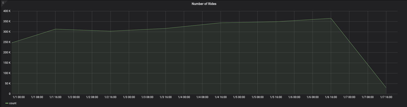
You can adjust the `time_bucket` function and compare the graphs:
```sql
SELECT
--1--
time_bucket('5m', pickup_datetime) AS time,
--2--
COUNT(*)
FROM rides
WHERE $__timeFilter(pickup_datetime)
GROUP BY time
ORDER BY time
```
When you visualize this query, it looks like this:

## Visualize geospatial data
Grafana includes a Geomap panel so you can see geospatial data
overlaid on a map. This can be helpful to understand how data
changes based on its location.
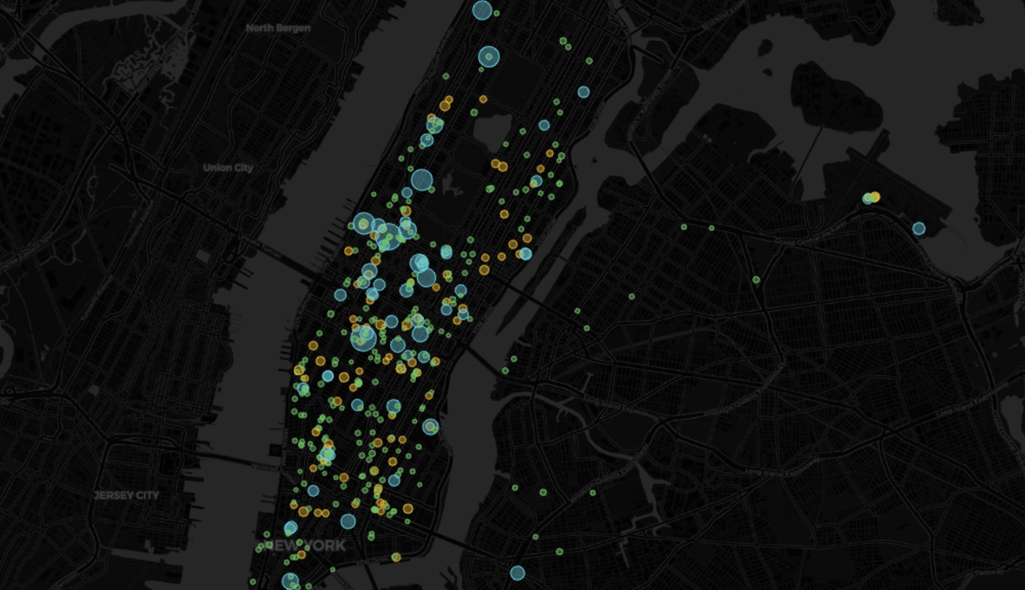
This section visualizes taxi rides in Manhattan, where the distance traveled
was greater than 5 miles. It uses the same query as the [NYC Taxi Cab][nyc-taxi]
tutorial as a starting point.
1. **Add a geospatial visualization**
1. In your Grafana dashboard, click `Add` > `Visualization`.
2. Select `Geomap` in the visualization type drop-down at the top right.
2. **Configure the data format**
1. In the `Queries` tab below, select your data source.
2. In the `Format` drop-down, select `Table`.
3. In the mode switcher, toggle `Code` and enter the query, then click `Run`.
For example:
```sql
SELECT time_bucket('5m', rides.pickup_datetime) AS time,
rides.trip_distance AS value,
rides.pickup_latitude AS latitude,
rides.pickup_longitude AS longitude
FROM rides
WHERE rides.trip_distance > 5
GROUP BY time,
rides.trip_distance,
rides.pickup_latitude,
rides.pickup_longitude
ORDER BY time
LIMIT 500;
```
3. **Customize the Geomap settings**
With default settings, the visualization uses green circles of the fixed size. Configure at least the following for a more representative view:
* `Map layers` > `Styles` > `Size` > `value`.
This changes the size of the circle depending on the value, with bigger circles representing bigger values.
* `Map layers` > `Styles` > `Color` > `value`.
* `Thresholds` > Add `threshold`.
Add thresholds for 7 and 10, to mark rides over 7 and 10 miles in different colors, respectively.
You now have a visualization that looks like this:
[nyc-taxi]: /tutorials/real-time-analytics-transport/
[grafana-website]: https://www.grafana.com
[time-buckets]: /use-timescale/time-buckets/
[grafana-self-managed]: https://grafana.com/get/?tab=self-managed
[grafana-cloud]: https://grafana.com/get/